Your LLM Inference Cluster Is Probably Operating Suboptimally

Why this problem, and why write about it

LLM inference is unarguably one of the most dominant workloads in the world. Let's say you are a company who wants to use Llama 3 70B or Qwen3 80B A3B for your AI product. You can do it by paying by API call. However, it is not realistic in terms of cost management. It is way too expensive, especially when your product grows with more users.

For this reason, once you reach a certain scale, you need to deploy your own inference infrastructure. How? Hmm, it becomes more of a headache.

Let's say you did it. Somehow you created a cluster with GPUs. Woah! Now how are you going to deploy the LLM? I am not talking about the mechanical process of running the containers, installing dependencies, etc. Yes, that is also a big pain, but even if everything is ready, there is one remaining really important question: "What cluster configuration are you going to use to serve the LLM at the best throughput and lowest cost?"

Let me give you a very concrete scenario to show how challenging it is to answer this question.

The spread between a good configuration and a bad one is not small like 10% — for the measurements we will show, it is routinely 2–5× on the same model, same workload, same cloud region. At the scale the industry is moving toward, 2–5× is real money. A team serving a 70B model at sustained load can quietly turn a misconfigured cluster into mid-six-figures of annual waste.

The waste is invisible for a reason: the numerator on the cost ratio (GPU-hours burned) looks normal, and the denominator (tokens served per dollar) is only meaningful relative to an optimum that nobody has computed. You cannot tell if you are paying a tax if you have never seen the untaxed price. (Maybe you are already.)

By the way, TL;DR: this is exactly the problem we at Tandemn are solving. Talk to us — we'll serve whatever model you want at the lowest cost and highest throughput possible, with our own advanced infrastructure stack that self-optimizes for your workload, your cluster, your SLO, and your cost budget.

---

Here is the analysis a reasonable engineer would be tempted to do first: read the GPU hardware specifications, compute $/TFLOPS and $/GB and $/(GB/s), and pick the GPU that is cheapest on whichever resource the roofline says dominates. Some will push it further by applying a roofline analysis on top.

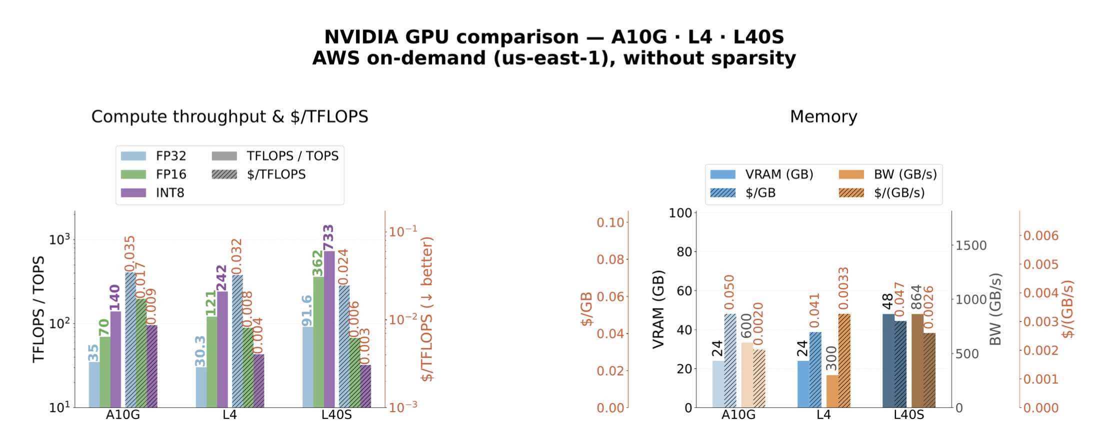Figure 1. NVIDIA A10G, L4, and L40S compared on AWS on-demand pricing (us-east-1), dense numbers (no sparsity). Left: compute throughput (FP32 / FP16 / INT8, solid bars) and $/TFLOPS (hatched, right axis — lower is better). Right: VRAM capacity and $/GB; memory bandwidth and $/(GB/s).

Three different GPUs win three different contests here. L40S is cheapest per FP16 TFLOP ($0.006 vs A10G's $0.017 — nearly 3× cheaper compute per dollar). L4 is cheapest per GB of VRAM ($0.041). A10G is cheapest per GB/s of memory bandwidth ($0.0020). Which one is right for your inference workload? The figure cannot tell you.

Worse, none of those three metrics predicts $/token. Each assumes the resource actually gets used — that the FLOPS run forward passes rather than all-reduce, that the bandwidth gets saturated during decode, that the VRAM is big enough to hold both the model and a real KV cache. Each of those assumptions can fail silently in practice, and when one fails, the spec-sheet math becomes fiction.

Before making any arguments about why it is structurally hard, let's see what happens when you try to predict a single throughput number for a single, fully-specified deployment.

---

The paradox: you cannot predict your own throughput

I would say, nope. It will be very difficult, unless you have a dedicated team for this job (or us at Tandemn 😉).

Take a 70-billion-parameter model. Put it on L40S GPUs. Run a fixed workload through vLLM. Now tell me what throughput you'll get.

You can't. Sorry — the question was incomplete.

How many L40S GPUs? 4 GPUs? 8 GPUs? And what's your parallelism strategy? What tensor-parallel and pipeline-parallel degrees? If the deployment spans nodes, what is the network between them — PCIe, NVLink, EFA? And what is the workload — are prompts 256 tokens long or 8,192? Are outputs 64 tokens or 2,048? Do prompts share prefixes? How much? What serving engine are you using? vLLM or SGLang? What version of vLLM?

Let's say this is your deployment plan.

Llama-70B, BF16, on four L40S GPUs in a single AWS g6e.12xlarge instance, TP=4 PP=1, vLLM 0.10 with chunked prefill on, 2,048-token inputs, 512-token outputs, no shared prefixes.

The question is now fully specified.

What would be the throughput for this deployment?

Probably it is still not easy to answer. And most people's first approach is to calculate it from the hardware specification plus a basic FLOP estimate for the given LLM.

For example, "an L40S has 362 TFLOPS of FP16 compute and 864 GB/s of memory bandwidth. So you can try to calculate throughput from the hardware specs."

Useful, but not an answer. We argue that this is the wrong way to solve the problem for two reasons. 1. The spec is the theoretical ceiling — definitely not what you'll actually observe. 2. You need to model the entire inference stack from hardware to serving engine and the LLM model and additionally all the factors that affect the throughput and cost. Practically not possible.

---

But let me still try the calculation. See if you agree.

Decode is memory-bandwidth-bound: every generated token requires streaming the full model shard from HBM once. The model is ~140 GB in BF16, sharded four ways at TP=4, so each L40S holds about 35 GB. At 864 GB/s, each GPU streams its shard in roughly 41 ms — about 24 tokens/second per sequence. A reasonable KV-cache budget on 48 GB cards lets you batch on the order of 64 concurrent sequences, so aggregate decode throughput lands around 1,500 tokens/second.

Prefill is compute-bound: 4 × 362 TFLOPS ÷ ~140 GFLOP per token ≈ 10,000 prefill tokens/second.

Blending the two for a 2,048-in / 512-out workload, a roofline suggests something in the neighborhood of 1,800–2,500 tokens/second sustained.

It is probably hard to trust. You know it is such a complex system that you never really know what happens at each layer of the stack and how the layers interact. You are right not to believe it — and you should not.

---

A quick tour of the stack — where the cost actually lives

The reason that it is so challenging to predict throughput up-front accurately is that it emerges from the interaction of all these independent factors.

The model. Dense or sparse (MoE)? 7B, 70B, or 235B? GQA ratio, layer count, context budget — each shifts feasibility, per-token FLOPs, KV footprint, and arithmetic intensity. Quantize to FP8 or INT8 and the memory footprint halves; on Hopper-class GPUs with native FP8 tensor cores, raw throughput changes too.

The inference engine. vLLM, SGLang, TensorRT-LLM. Each exposes knobs that move throughput by double-digit percent: chunked prefill overlaps prefill/decode phases (20–40% gain on prefill-heavy workloads), prefix caching skips shared-prefix recomputation, max_num_seqs caps concurrency and KV pressure, gpu_memory_utilization trades VRAM headroom for batchable sequences, kv_cache_dtype halves KV footprint at small accuracy cost.

The GPU. FP16 FLOPs, memory bandwidth, VRAM, tensor-core generation, interconnect. A10G: 70 TFLOPs, 600 GB/s, 24 GB. L40S: 362 TFLOPs, 864 GB/s, 48 GB. H100: 989 TFLOPs, 3,350 GB/s, 80 GB with NVLink. Specs alone don't give you the ranking — interconnect (PCIe vs NVLink), virtualization (bare metal vs AWS's virtualized PCIe on g6e), and VRAM-bound KV capacity all shift it.

Parallelism. TP shards weights and all-reduces at every layer; PP pipelines consecutive layers across GPUs (cheaper comm, but pipeline-bubble overhead); DP replicates. Hard constraints: TP divides attention and KV head counts, PP divides the layer count, TP × PP × DP fits the cluster. The right choice depends on interconnect (NVLink tolerates higher TP, PCIe saturates earlier) and workload shape (short decode tolerates bubbles, long decode doesn't).

Workload shape. Input/output token ratio decides whether you're compute-bound (long prefill, short decode) or memory-bandwidth-bound (short prefill, long decode). Same cluster sits in a different bottleneck regime depending on what your users type that day. RAG with 8k context and 512-token answers is not the same job as creative writing with 256-in, 2k-out — and the cost-optimal hardware isn't the same either.

The KV cache. The silent VRAM consumer. For a 70B GQA model, one 2,048-token sequence takes ~600 MB of KV; 64 concurrent sequences take ~40 GB. In practice, the KV cache — not the model weights — decides how many requests run concurrently, which decides how close you get to hardware throughput.

Each one moves throughput on its own and also in a reciprocal way. Any analytical argument that treats them independently is wrong — because in practice the bottleneck (compute, memory bandwidth, KV cache, or all-reduce) shifts between axes depending on the other axes. These are only six axes, but there are even more factors.

---

Let Me Ask Claude

Nahh, we have Opus 4.7 now. I'll just ask it. Problem solved.

Are you thinking "Nah, I won't bother. I'll just ask an LLM."? Okay, let's do that.

Claude Opus 4.7 says: Input (prefill): ~4,000 tok/s
Output (decode): ~1,000 tok/s
Total: ~5,000 tok/s

Gemini Pro says: Total Throughput: ~2,000 to 2,500 tokens/sec
Input (Prefill) Throughput: ~1,600 to 2,000 tokens/sec
Output (Decode) Throughput: ~400 to 500 tokens/sec

I measured the same configuration. It sustains 532 tokens/second. So Gemini Pro was optimistic by roughly 4×, and Claude Opus 4.7 was optimistic by roughly 9×.

Maybe you can achieve 2000 tokens/second at a specific system. Who knows. It strengthens our point that it is not easy to predict the throughput accurately without running the workloads on the cluster that you are going to use.

---

Conclusion

You have tried the three things any reasonable engineer would try — vendor specs, roofline math, frontier LLM — and you still do not know your sustained throughput within 2× of ground truth for a single fully-specified deployment.

And I haven't even touched the parts where the answer changes depending on workload shape, where the cost-optimal configuration is not the throughput-optimal one, or where adding more GPUs on the same cloud instance makes aggregate throughput go down. Those are ahead.

In the real world, it is even more complex. There are dozens of factors that affect the throughput and cost.

In Part 2, we show the full sweep benchmark results done in a real cluster.

Stay tuned.