Introducing Koi: Get More from the GPUs You Already Have
Tandemn
In collaboration with NVIDIA, ByteDance, UC Berkeley, UIUC, and NYU
Executive Summary
Get more from the GPUs you already have. Tandemn learns how models behave across GPU types and configurations, then plans the fleet as a whole across cloud providers and regions. By placing online and batch jobs on suitable available capacity, it puts fragmented and underused compute to work while balancing throughput, cost, latency targets, and deadlines. That creates room to admit more jobs and serve more demand without expanding your infrastructure.
More throughput. Lower cost per token. More jobs admitted.
-
45%
More throughput
-
31%
Lower cost per token
-
95.65%
Online jobs admitted
Throughput and cost improvements are compared with the strongest baseline; 95.65% of online jobs and 100% of batch jobs were admitted.
1 Introduction
An LLM inference fleet must continually place and configure a changing mix of active and pending jobs. Each job specifies a model, workload profile, class (online or batch), and serving target, while deployments span environments defined by cloud, region, market, and hardware. These decisions must be revised as jobs arrive, complete, and cluster capacity changes, and they cannot be inferred reliably from hardware or topology alone.
For a profiled 70B model, feasible deployments on the same accelerator family vary by in throughput and in cost per token. The best configuration also shifts with workload shape, traffic patterns, and serving-stack changes; engine, driver, and collective-library updates alone can move throughput by 10–30% for an otherwise unchanged deployment. As workloads drift, a configuration that was previously optimal can therefore become inefficient or fail to meet its serving target. A configuration profiled once therefore cannot remain optimal, motivating online calibration.
Existing systems solve parts of this problem. Serving engines optimize request execution; orchestrators provision and replicate services; per-job optimizers search configurations independently; and serving planners and cluster schedulers optimize placement or resource allocation. No existing system jointly chooses deployment configuration and cluster allocation for co-located online and batch jobs across a heterogeneous, multi-cloud fleet.
These decisions become coupled when jobs compete for finite resources. A planner that optimizes jobs independently may allocate a scarce accelerator to a job with a workable alternative while blocking one with none. In our three-hour simulation benchmark, PRISM achieves 765 goodput tok/s at dollars/token, while Koi’s cluster-wide planning reaches 2,911 tok/s at dollars/token— higher goodput at 74% lower cost per token.
Joint optimization also requires predicting unseen deployments. Analytical models are efficient but brittle to memory, communication, and engine behavior. Language models can narrow the search but do not provide calibrated estimates: in our measurements, two frontier models overpredict throughput by and , while a roofline model errs by up to . Measurement-driven methods avoid explicit models but require repeated trials that consume serving capacity.
Koi bridges these approaches with an uncertainty-aware causal representation linking deployment decisions, runtime mediators, and serving outcomes. Each causal edge carries confidence updated from supporting or contradictory deployment evidence, while predictions retain uncertainty about their accuracy. High-confidence relationships support exploitation; uncertain relationships identify informative deployments to test but increase estimated risk. Scoped mechanisms compose related edges into reusable hypotheses across workloads, configurations, and environments. Each deployment therefore updates both what Koi believes about inference behavior and how strongly those beliefs should guide future plans.
A language model proposes candidate deployments using the causal graph, cluster snapshot, workload, and matching evidence. Deterministic components then predict candidate behavior, score it against job objectives, compose candidates into a cluster-wide plan, and enforce capacity, SLO-risk, and reconfiguration constraints. Only deployment evidence updates causal confidence, and only deterministic components perform prediction, scoring, feasibility checking, selection, and commitment. This separation lets Koi use language-model reasoning to explore a combinatorial search space without allowing model output to override measured evidence or cluster constraints.
We evaluate Koi on simulated and real-world clusters against baselines spanning queuing policies, per-job optimizers, placement solvers, evolutionary search, and unstructured language-model planners. On the three-hour benchmark, Koi outperforms every baseline on all reported metrics. Ablations show that the gains come primarily from the control structure around the language model: deterministic evaluation adds 16.3 composite-score points over language-model planning alone, and Koi’s persistent evidence state adds a further 19.2 points.
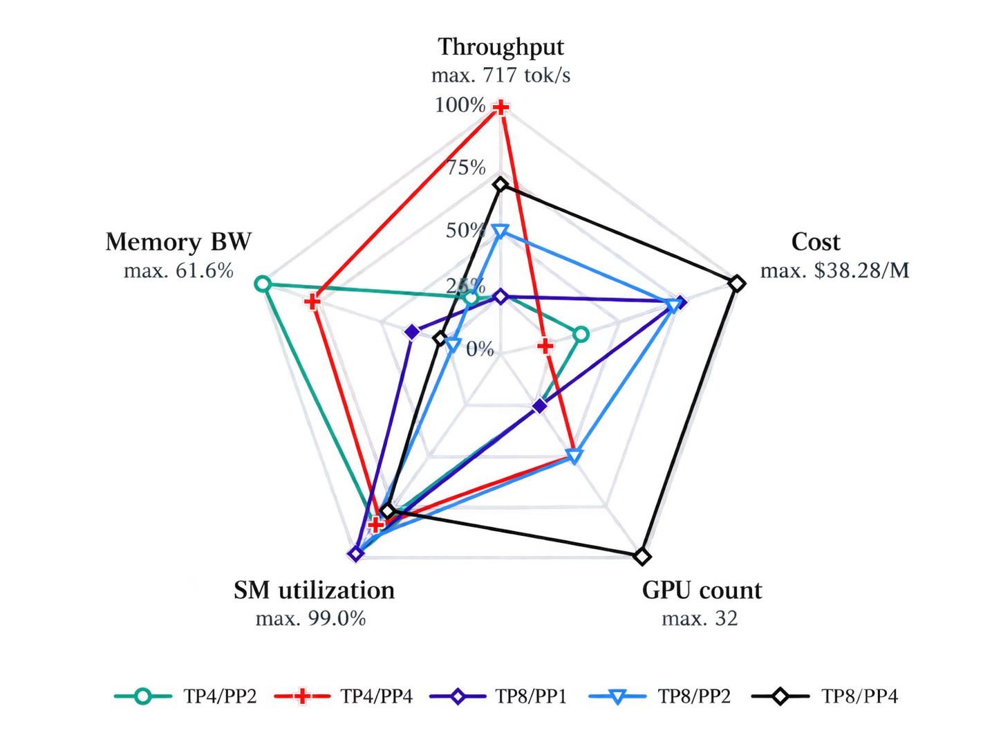
Deployment tradeoffs. Feasible configurations for the same model can produce very different throughput, cost, memory utilization, and GPU use, so a single static profile is not enough.
2 Koi
2.1 Overview
Each tick, Koi executes an eight-stage closed loop that updates evidence from the cluster and searches for a better cluster-wide plan. States S0–S3 refresh the planner state by snapshotting jobs, placements, and capacity (S0), collecting per-rank telemetry (S1), comparing observations against stored predictions (S2), and updating the evidence state (S3). Planning begins at S4, where the agent proposes a cluster-wide action for each job: place, reconfigure, retain, or defer. Deterministic evaluation at S5 scores the proposal against job-specific performance, expected evidence, SLO risk, and reconfiguration cost, and validates constraints C1–C5. Invalid or non-improving plans return to S4 with scores and diagnostics. Once the search budget is exhausted, Koi commits the best feasible cluster-wide plan (S6) and closes the loop (S7).
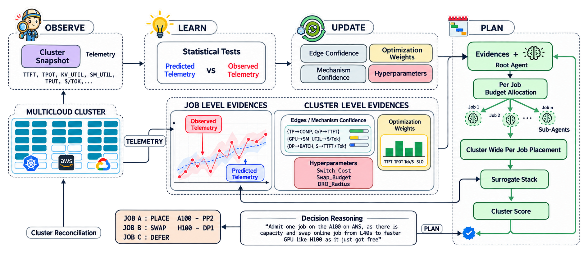
Koi architecture. Koi observes the fleet, compares predictions with telemetry, updates its evidence, and plans the next cluster-wide placement through a deterministic validation and scoring layer.
2.2 Problem formulation
At each planning tick, Koi selects deployments for the cluster’s active and pending jobs. Each job has a workload profile and serving target —a latency bound for online jobs or a completion deadline for batch jobs—while describes the available capacity across environments.
A deployment follows four levels. A chain is one model copy running in environment under configuration . A rank contains homogeneous replicas of that chain. A job’s ladder is the set of ranks assigned to it, and the cluster plan contains one ladder for every active and pending job. Keeping the previous ladder retains an active deployment, while defers a pending job.
Each ladder produces five outcomes: cost per token, p99 TTFT, p99 TPOT, throughput, and SLO margin. Job-specific weights express the relative importance of these objectives. Koi combines them using an augmented Tchebycheff score:
where is the normalized gap between the predicted outcome and job ’s reference point.
At each tick, Koi seeks a cluster-wide plan that maximizes aggregate job value while discouraging unnecessary reconfiguration:
A feasible plan must satisfy five constraints: C1, all ladders fit available cluster capacity; C2, each chain is physically valid with respect to VRAM and parallelism; C3, predicted SLO-breach probability remains below ; C4, no more than active jobs are reconfigured in one tick; and C5, job quotas and priorities are respected. Pending jobs may therefore be deferred even when a deployment is technically feasible.
If the outcomes of every candidate ladder were known, this program would directly define the best plan. In practice, deployment behavior is uncertain and changes over time. Koi therefore predicts outcomes from accumulated evidence, deploys selected plans, observes their behavior, and uses those observations to improve subsequent decisions.
2.3 Mechanisms and predictions
To make deployment behavior testable and transferable, Koi represents inference as a directed acyclic graph, , where contains planner-controlled decisions (hardware, engine, parallelism, quantization, batching, routing), contains telemetry-derived runtime mediators (KV-cache utilization, pipeline bubbles, communication latency, memory pressure, SM utilization), and contains the serving outcomes defined above. Only and edges are permitted, ensuring every modeled effect passes through telemetry; the registered edge set is fixed at initialization.
Each edge maintains a belief , where and accumulate supporting and contradictory evidence, and is its confidence. Because the same confidence can reflect different amounts of evidence, Koi also tracks normalized posterior uncertainty:
Exploration prioritizes edges with high , where additional deployment evidence is most informative.
Edges compose into scoped hypotheses called mechanisms. A mechanism pairs a connected subgraph with an applicability scope over models, hardware, workloads, and conditions, a natural-language statement , and Beta state . The LLM proposes mechanisms, which are admitted only if they form a valid, non-duplicate path over registered edges and are initialized with .
Both and , the predicted mediator and outcome values, come from a deterministic surrogate. Given a job’s workload profile and one candidate ladder, it composes operator-level latency profiles with a replay simulator to predict p99 TTFT, p99 TPOT, and throughput. The remaining mediators and outcomes are derived from those predictions, the job’s targets, and the allocation price carried by . When a model has no measured profile, it substitutes the nearest profiled architecture on that hardware and rescales by its measured prefill and decode speed ratios.
The surrogate is an approximation, so Koi carries prediction uncertainty into planning and rejects ladders with under C3. A deployed ladder tests every mechanism whose scope it satisfies by comparing predicted mediator and outcome trajectories against observations. For either trajectory , Koi defines the residual at observation as and accumulates it in a two-sided cumulative sum detector:
with slack , declaring divergence when or for threshold , where is the empirical residual scale. Accumulating the residual rather than thresholding each sample separates persistent prediction error from isolated deviations.
CUSUM assigns each mechanism evaluation to one of four quadrants: Q1, mediators and outcomes both match; Q2, mediators match and outcomes diverge; Q3, mediators diverge and outcomes match; and Q4, mediators and outcomes both diverge. Q1 adds supporting evidence, Q4 contradictory evidence, and Q2–Q3 update edges according to their invariant causal prediction result. The self-calibration loop uses the Q1 rate to adapt exploration.
2.4 Scoring a plan
Because Koi scores predicted rather than known outcomes, it augments the cluster program with two terms: risk from prediction error and exploration value from testing uncertain causal relationships. Exploitation, risk, and switching cost sum over jobs; exploration is scored once per plan to avoid double-counting repeated tests.
Exploitation
Exploitation is the per-job augmented Tchebycheff score evaluated on the ladder’s aggregated outcomes. High-confidence causal relationships guide exploitative candidates, while favors those whose predicted outcomes best match the job’s weighted priorities.
Exploration
Exploitation alone favors deployments the surrogate already predicts to be good, so relationships that have never been exercised stay untested. Exploration rewards a plan for testing uncertain edges and mechanisms:
where indicates whether any ladder in exercises edge , and analogously for mechanisms. Mechanisms, weighted by , are scored separately because their scope can fail even when each constituent edge is well supported.
Risk
A surrogate is most likely to be wrong when conditions have shifted, which is also when a plan is most likely to breach an SLO. Koi therefore evaluates each prediction against a band rather than a point. Let be the historical residuals for objective and their empirical standard deviation. The band is:
The quantile terms carry the observed error distribution and the terms inflate it, with in the role of a Wasserstein ambiguity radius rather than as the solution to a distributionally robust program. Koi calibrates from realized coverage, widening it when outcomes fall outside the band more often than the target rate and tightening it as calibration improves.
From the band, Koi estimates the probability that each SLO-constrained objective is violated, and combines them as:
where is the set of objectives constrained by . Treating those objectives as independent is conservative, since latency violations are positively correlated in practice, so the product understates the joint satisfaction probability and overestimates risk.
Switching cost
The reconfiguration cost for job is decomposed into four components:
All terms are zero for an unchanged ladder. captures loading and warm-up, concurrent execution, draining and termination, and transient underperformance. The penalty adapts to the observed reconfiguration rate to discourage unnecessary migrations. Separately, the swap budget imposes the hard C4 cap on how many active jobs may change ladders in one tick.
Cluster score
The four terms combine into a single plan score:
Koi aims to select the highest-scoring feasible plan:
where is the set of plans satisfying C1–C5. Exhaustive maximization is infeasible and the per-tick search is budgeted, so Koi commits the highest-scoring feasible plan it finds rather than the maximizer. The exploration weight and switching penalty are adapted by the slow loop; the risk weight is fixed.
2.5 Self-calibration
Koi adapts the quantities that govern planning from how well its predictions have held. Edge and mechanism confidence update every tick. On a slower schedule, Koi adjusts the exploration weight , swap budget , switching penalty , robustness radius , ideal point , and CUSUM thresholds, each from accumulated residuals.
Most of these follow one signal. Let be the fraction of decided evidence–mechanism pairs over a rolling window of ticks that fall in Q1, and with let the regret signal be:
which increases as predictions become less reliable. Regret is derived from the Q1 rate: a high regret signal indicates poor configurations and motivates continued exploration. The exploration weight is:
with target regret and adaptation rate . The same signal raises the swap budget when predictions are unreliable, so more active jobs may be reconsidered. The switching penalty instead follows the observed reconfiguration rate, rising as churn grows to damp thrashing.
The radius follows realized coverage, widening when outcomes fall outside the band more often than the target rate and tightening otherwise. The ideal reference tracks the best outcomes a job has achieved:
where is job ’s deployment history and a margin that preserves dominance.
2.6 Agentic planner
The search space for a cluster deployment is combinatorial and coupled. Jobs compete for finite resources under different workload profiles and SLOs, and each configuration consumes resources another job might need. To navigate this search space, Koi uses an LLM to query the causal DAG and reason over mechanisms when proposing configurations, while deterministic code evaluates, scores, and selects among them.
A root planner receives the frozen cluster snapshot and assigns each job a budget book, a soft upper bound on which GPU types and instance pools the job may consider. Budgets can overlap, and contention is resolved later by a capacity-constrained solver that assigns at most one ladder per job to the available GPUs. The root planner invokes per-job specialist sub-agents to propose candidate ladders within each job’s budget. Each specialist receives the job’s model architecture, workload profile, current deployment, budgeted hardware, and all mechanisms whose scope matches the job. It can query the DAG backward: given a target SLO, the specialist traces which decisions affect it through which mediators, focusing on the decisions that matter.
These proposals are advisory. Koi first validates each candidate for physical feasibility, then invokes the surrogate to predict and score its performance. The resulting ladders compete for finite capacity under the joint selector, which assigns at most one ladder per job to maximize cluster-wide gain while accounting for unserved demand, improvement over active deployments, and switching cost. The root planner may inspect the result and propose additional candidates, but cannot override deterministic scores, capacity checks, or constraints C1–C5.
3 Evaluation
Our evaluation asks three questions. First, how does Koi compare with static, classical, outcome-learning, evolutionary, and language-model planners in goodput, SLO attainment, admission, and cost? Second, do joint optimization, evidence accumulation, and health-triggered recovery operate as intended, and how do these effects change with deployment scale and duration? Third, what do deterministic planning tools, the causal evidence graph, and cross-tick learning contribute, and how sensitive are the results to the language-model backbone?
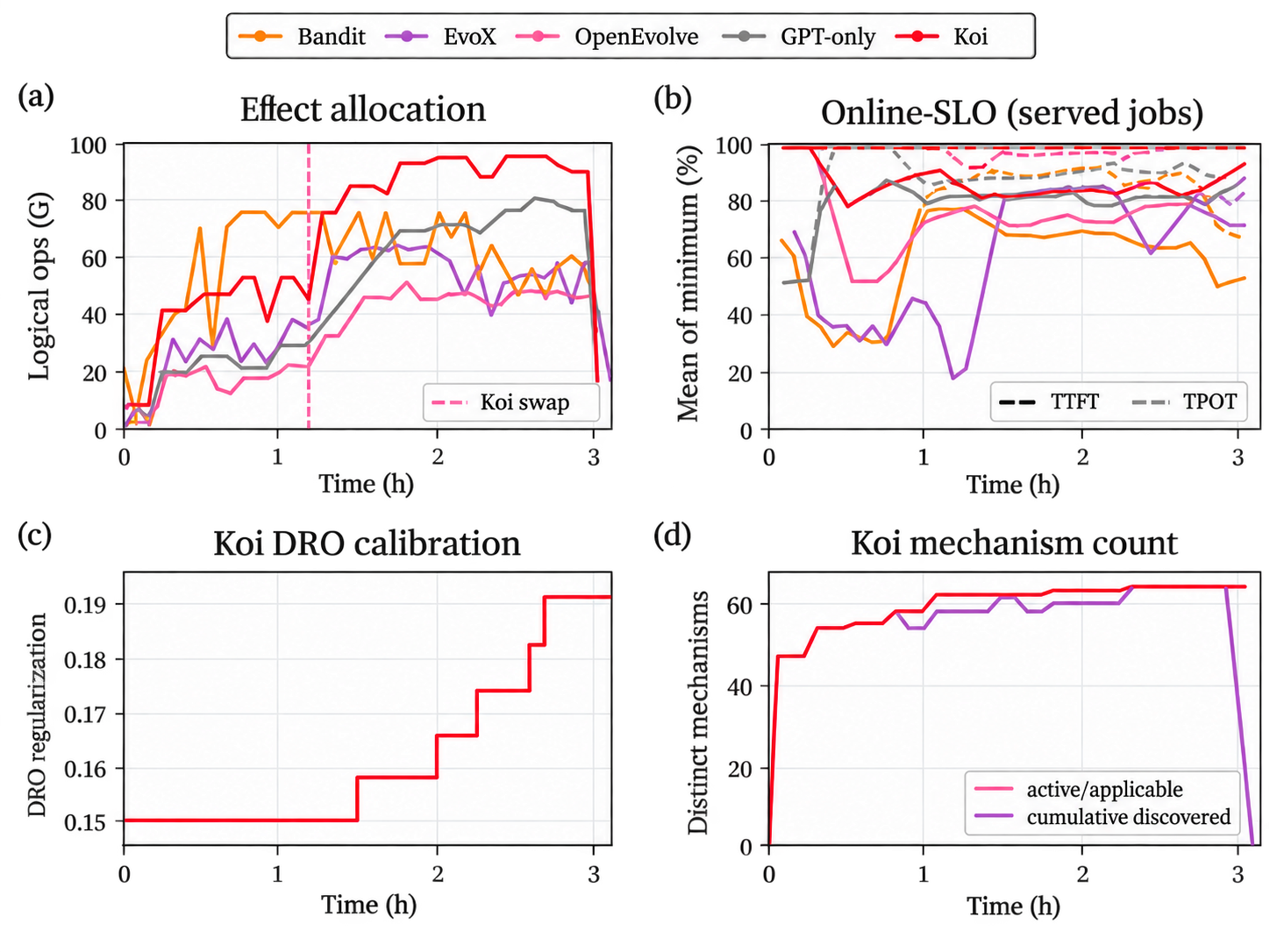
Evaluation traces. Over a three-hour heterogeneous run, Koi improves fleet allocation, online SLO attainment, calibration, and the number of useful mechanisms discovered as evidence accumulates.
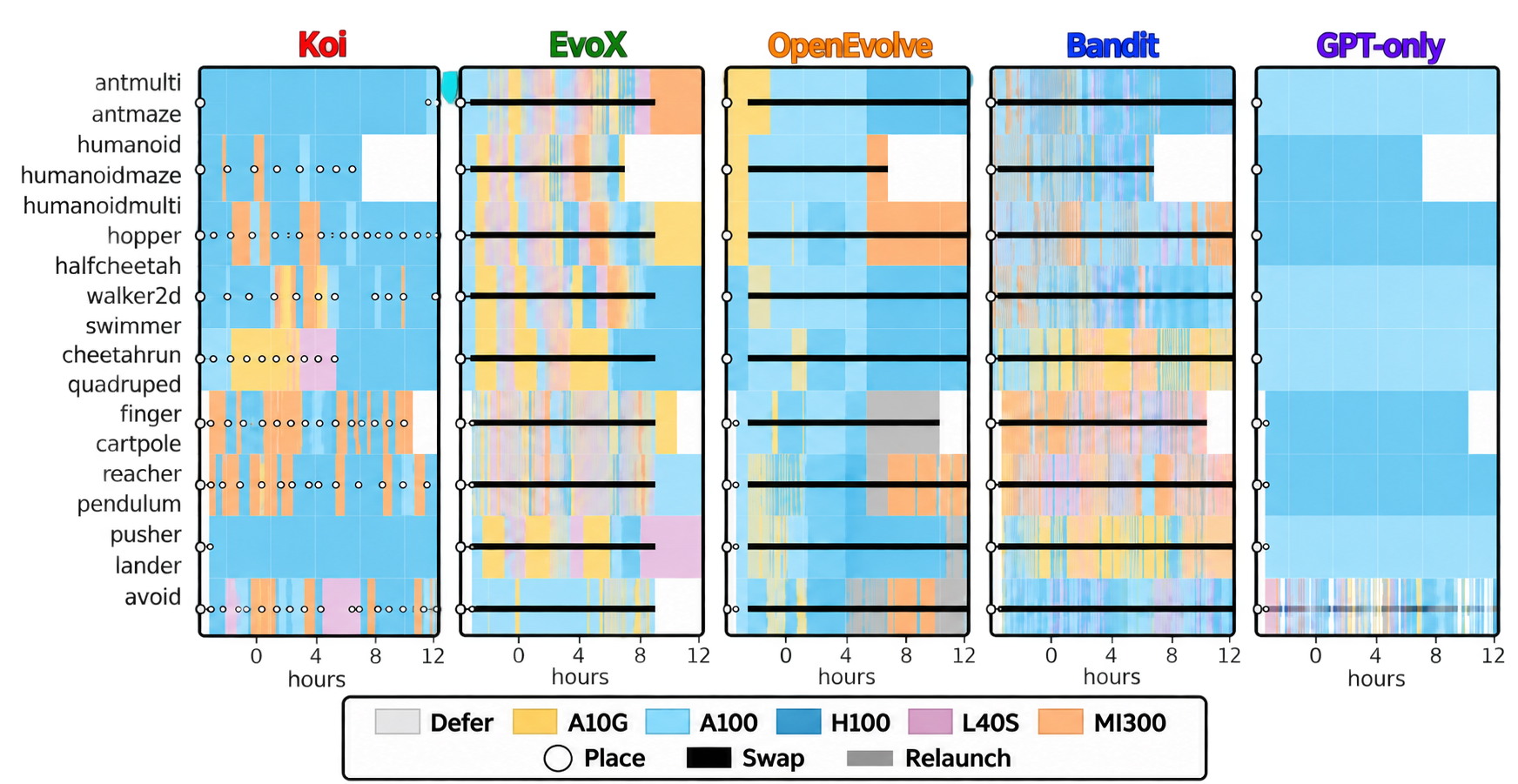
Switching and service stability. Koi concentrates changes around meaningful placement decisions while maintaining strong online service-level performance instead of constantly reshuffling the fleet.
3.1 Experimental setup
Benchmarks. We evaluate Koi on one real-hardware and three simulated benchmarks: a three-hour deployment on a 104-GPU heterogeneous GCP cluster, three-hour and 12-hour heterogeneous simulations, and a 12-hour homogeneous simulation. Each benchmark runs the same concurrent mix of 25 online and batch workloads across ten model architectures spanning 1B to 235B parameters, including dense and mixture-of-experts models. Workloads range from short moderation requests to 24K-token long-context summaries and decode-heavy agentic tasks; six batch jobs have deadlines between 20 and 135 minutes. Traffic follows Poisson, constant, and gamma arrival processes derived from production-style workload profiles.
Baselines. We compare Koi against ten schedulers spanning five approaches: non-learning policies (FCFS + First-Fit, EDF, and Best Fixed), per-job optimization (PRISM), global optimization without mechanism learning (Rolling CP-SAT and contextual Thompson sampling), LLM-guided planning (GPT-only and an agentic planner with inspection and validation tools), and evolutionary search (Rolling EvoX and OpenEvolve). Each baseline receives the same cluster snapshots, candidate catalog, resource constraints, and safety checks. LLM-based policies use GPT-5.6-Luna for the main comparison; we separately evaluate Koi with different LLM backbones.
Metrics. A common evaluator computes all results from per-run traces using workload-defined denominators, so a planner cannot improve its score by refusing or dropping work. We report online and batch admission, batch progress, TTFT and TPOT SLO attainment, SLO-honoring goodput, and cost per SLO-token. Goodput counts output tokens from online requests meeting both latency targets and from batch jobs meeting their deadlines; cost includes the full provisioned fleet, including idle capacity.
For a single summary measure, we use the geometric mean of three equally weighted pillars: Quality (TTFT, TPOT, and deadline attainment), Coverage (online admission, batch admission, and batch progress), and Efficiency (goodput and cost per SLO-token). Stochastic planners report results over at least three runs.
3.2 End-to-end performance
Heterogeneous simulations
Simulated benchmark results for 3-hour (400-GPU) and 12-hour (800-GPU) heterogeneous workloads. Values are stacked as 3-hour over 12-hour.
| Method | Hrs | Batch progress | Online admit | Batch admit | Cost/token (10⁻⁴ dollars) | TTFT met | TPOT met | Goodput tok/s | Overall |
|---|---|---|---|---|---|---|---|---|---|
| FCFS + first-fit | 3 12 | 57.71% 38.69% | 77.78% 78.26% | 57.14% 50.00% | 2.95 6.09 | 3.90% 2.45% | 6.89% 6.27% | 1,830.84 1,772.01 | 49.13 31.46 |
| Best fixed configuration | 3 12 | 57.71% 24.54% | 66.67% 69.57% | 57.14% 57.14% | 2.91 29.65 | 5.24% 7.63% | 13.61% 13.55% | 1,857.31 364.03 | 50.24 17.59 |
| EDF + first-fit | 3 12 | 57.71% 38.62% | 77.78% 78.26% | 57.14% 50.00% | 2.94 6.09 | 4.05% 2.36% | 7.27% 6.21% | 1,833.16 1,771.49 | 49.27 31.40 |
| Rolling CP-SAT | 3 12 | 41.99% 14.99% | 72.22% 78.26% | 57.14% 64.29% | 6.69 40.18 | 3.00% 2.89% | 15.88% 16.83% | 807.03 268.57 | 31.90 15.83 |
| Contextual bandit | 3 12 | 44.42% 30.52% | 66.67% 65.22% | 57.14% 50.00% | 5.43 14.16 | 8.09% 9.56% | 27.08% 23.06% | 993.08 762.20 | 37.49 24.89 |
| PRISM | 3 12 | 42.55% 15.35% | 77.78% 73.91% | 57.14% 64.29% | 7.06 57.66 | 2.80% 1.94% | 5.16% 4.69% | 764.66 187.18 | 29.06 11.14 |
| Rolling EvoX | 3 12 | 57.71% 50.71% | 66.67% 65.22% | 57.14% 64.29% | 2.69 3.37 | 9.90% 11.96% | 22.10% 24.02% | 2,004.06 3,012.00 | 54.34 50.01 |
| OpenEvolve | 3 12 | 56.70% 25.01% | 66.67% 78.26% | 57.14% 64.29% | 4.74 26.24 | 5.22% 9.19% | 23.41% 16.83% | 1,139.00 411.25 | 41.74 19.84 |
| GPT-Only (non-agentic) | 3 12 | 52.04% 17.54% | 77.78% 69.57% | 71.43% 71.43% | 6.31 16.86 | 3.98% 3.02% | 18.98% 17.29% | 855.60 640.25 | 35.28 21.34 |
| Koi | 3 12 | 84.55% 49.61% | 94.44% 95.65% | 71.43% 100.00% | 1.85 3.39 | 28.79% 27.95% | 41.80% 35.80% | 2,910.64 3,184.15 | 70.83 63.13 |
| Δ vs. best baseline | 3 12 | +26.84pp -1.10pp | +16.66pp +17.39pp | +0.00pp +28.57pp | +31.23% -0.59% | +18.89pp +15.99pp | +14.72pp +11.78pp | +45.24% +5.72% | +30.35% +26.23% |
Over three hours, Koi achieves 2,911 goodput tok/s, 45.24% more than the strongest baseline, while reducing cost per token by 31.23%; it also improves batch progress by 26.84 percentage points and TTFT/TPOT SLO attainment by 18.89/14.72 points. Over twelve hours, Koi admits 95.65% of online jobs and all batch jobs, improves goodput by 5.72%, and leads TTFT/TPOT attainment by 15.99/11.78 points, while batch progress is 1.10 points below EvoX and cost is 0.59% higher. Koi’s gain does not come from maximizing one workload class: it sustains more admitted work and substantially better online latency while remaining competitive on batch progress and cost.
Real-hardware cluster
| Method | Batch progress | Online admit | Batch admit | Cost/token (10⁻⁴ dollars) | TTFT met | TPOT met | Goodput tok/s | Overall |
|---|---|---|---|---|---|---|---|---|
| Contextual bandit | 50.00% | 53.33% | 100.00% | 0.45 | 22.23% | 33.66% | 2,291.03 | 51.05 |
| Rolling EvoX | 50.00% | 80.00% | 100.00% | 0.44 | 28.08% | 35.48% | 2,348.15 | 54.90 |
| OpenEvolve | 75.00% | 100.00% | 100.00% | 0.30 | 65.66% | 91.41% | 3,497.43 | 84.44 |
| Koi | 100.00% | 100.00% | 100.00% | 0.24 | 79.05% | 99.11% | 4,119.51 | 94.50 |
Against the best baseline, Koi improves batch progress by 25 points, cost by 20%, TTFT attainment by 13.39 points, TPOT attainment by 7.70 points, goodput by 17.79%, and the overall score by 11.91%.
Homogeneous 12-hour simulation
| Method | Batch progress | Online admit | Batch admit | Cost/token (10⁻⁴ dollars) | TTFT met | TPOT met | Goodput tok/s | Overall |
|---|---|---|---|---|---|---|---|---|
| Best fixed | 37.58% | 60.87% | 42.86% | 3.56 | 24.38% | 31.09% | 2,147.77 | 50.69 |
| Contextual bandit | 1.89% | 43.48% | 7.14% | 14.04 | 10.32% | 10.95% | 544.34 | 14.59 |
| Rolling EvoX | 14.92% | 65.22% | 14.29% | 4.76 | 29.61% | 37.10% | 1,606.39 | 40.37 |
| OpenEvolve | 14.92% | 65.22% | 14.29% | 6.76 | 20.26% | 32.46% | 1,130.77 | 33.18 |
| GPT-only | 40.06% | 65.22% | 57.14% | 4.29 | 18.15% | 33.62% | 1,783.61 | 49.17 |
| Koi | 36.62% | 78.26% | 57.14% | 3.51 | 31.37% | 39.29% | 2,175.63 | 56.68 |
3.3 Design evaluation
Joint optimization. In the real-cluster run, a Qwen3-235B job arrives while ten services are active. Admitting it would require reducing a Phi-4 service from two TP2 RTXPRO6000 replicas to one, cutting modeled capacity from 1,572 to 786 tok/s—below its 834 tok/s requirement—while its p99 TTFT already exceeds its target. Koi rejects the reclaim, defers Qwen for two ticks, and admits it after another batch finishes. The ten-minute delay avoids degrading an existing service without sacrificing eventual admission.
Evidence improves calibration. Across the 12-hour heterogeneous simulation, mean causal uncertainty falls by while learned residual corrections become more frequent and more accurate. As evidence accumulates, the median DRO radius contracts from 0.379 to 0.260, then widens again after a late workload shift. At larger scale and longer duration, Koi also accumulates substantially more evidence and decisive mechanism tests. Repeated deployments increase confidence under stable conditions while allowing exploration and robustness to rise again when behavior changes.
Recovery from degraded deployments. In the real cluster, a Mixtral service becomes unhealthy after only one of two A100-80GB replicas materializes, pushing p99 TTFT to 2,299 ms against a 700 ms target. A per-job sub-agent proposes a launchable TP8 A100 replacement, deterministic evaluation selects the swap, and the joint planner leaves all other active jobs unchanged. The request-level TTFT pass rate rises from 2.4% to 99.9%, and the service is healthy again within three ticks.
Balancing exploration and exploitation. Koi produces long stable placement intervals, with changes concentrated on degraded services. EvoX and the contextual bandit instead produce dense swap sequences, while OpenEvolve and GPT-only largely preserve their initial placements. Across the trace, Koi issues 201 swaps and 2,076 keeps, compared with 1,464 swaps for EvoX and 1,928 for the bandit. Koi therefore avoids both repeatedly perturbing productive deployments and leaving poor initial placements uncorrected.
3.4 Ablation study
Koi sub-components
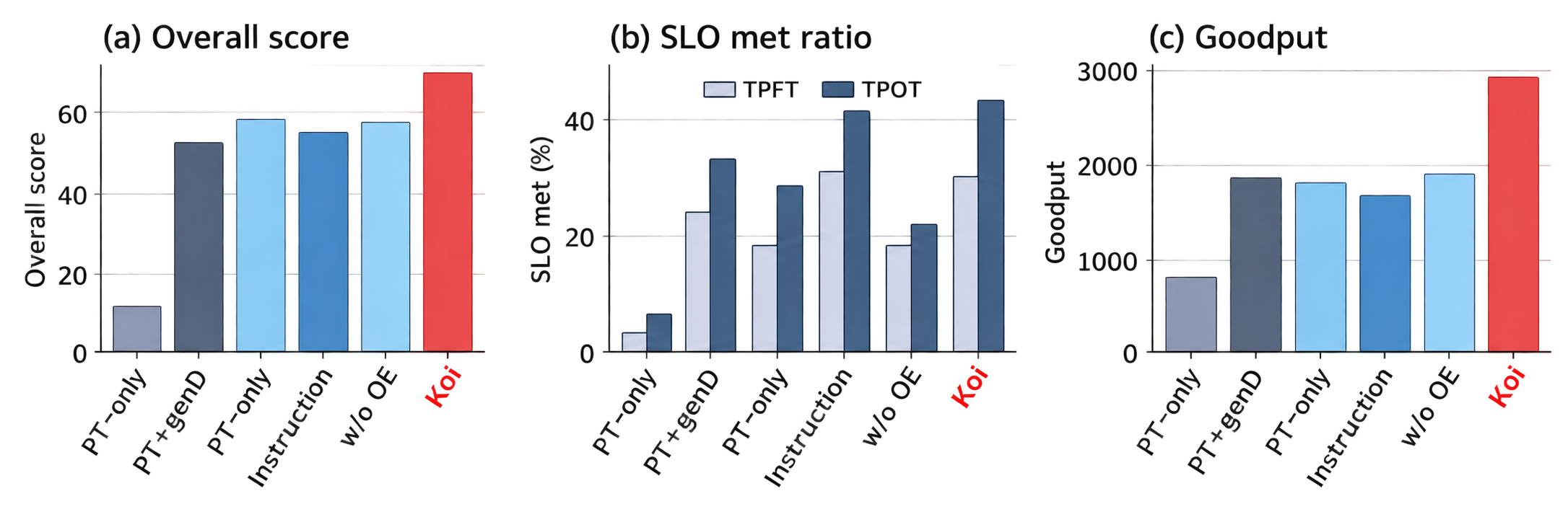
Ablation results. Removing deterministic tools, the causal evidence graph, or online learning reduces the system’s ability to combine throughput, cost, batch progress, and latency performance.
| Variant | Batch progress | Online admit | Batch admit | Cost/token (10⁻⁴ dollars) | TTFT met | TPOT met | Goodput tok/s | Overall |
|---|---|---|---|---|---|---|---|---|
| GPT-only | 52.04% | 77.78% | 71.43% | 6.31 | 3.98% | 18.98% | 855.60 | 35.28 |
| Opencode SDK (GPT-5.6-Luna) | 54.77% | 88.89% | 57.14% | 2.95 | 25.74% | 32.62% | 1,826.64 | 51.55 |
| Koi without DAG/mechanisms | 59.42% | 94.44% | 100.00% | 3.05 | 21.66% | 38.33% | 1,770.03 | 58.34 |
| Koi without online learning | 63.01% | 94.44% | 85.71% | 3.33 | 16.49% | 37.74% | 1,621.48 | 54.79 |
| Full Koi | 84.55% | 94.44% | 71.43% | 1.85 | 28.79% | 41.80% | 2,910.64 | 70.83 |
Giving the language model deterministic prediction, scoring, and validation tools increases goodput from 856 to 1,827 tok/s, raises TTFT attainment from 3.98% to 25.74%, and reduces cost per token from to . The complete system reaches 2,911 tok/s; removing the causal graph reduces goodput to 1,770 tok/s, while freezing online updates reduces it to 1,621 tok/s. Full Koi also completes 84.55% of batch work, versus 59.42% without the graph and 63.01% without online learning, despite admitting fewer batch jobs than either variant. Deterministic tools ground each planning attempt, while persistent mechanism evidence improves which valid plans are retained and revisited across ticks.
LLM backbone
The backbone ablation localizes the Cohere–GPT-5.6 Sol difference to a single 7,200-request Llama-70B batch campaign. Both planners admit it at 00:15 and never reconfigure it, but Cohere selects one eight-GPU MI300 TP8 chain and finishes at 01:07 with 82 minutes of deadline slack, whereas Sol selects four TP4 A100 replicas using 16 GPUs and reaches 7,115 requests by the 02:30 deadline, missing by 85. Because batch goodput credits the campaign only when it meets its deadline, this single decision contributes 8.64 million tokens and explains 99.3% of their trace-derived goodput gap; their online contributions differ by only 57,921 tokens.
Deterministic validation bounds the action space but cannot make all valid candidates equally useful: a small number of initial proposals can dominate the final result. This single-run comparison does not isolate accelerator type, parallelism, replication, or batching limits, which change together.
The achieved outcomes—TTFT, TPOT, and the other job metrics—of all jobs in all ablations are well within three standard deviations of each other, indicating model-agnostic behavior.
4 Conclusion
LLM inference planning is a moving target: the best deployment depends not only on model and hardware, but also on workload shape, competing jobs, and how well prior predictions hold. Koi addresses this by combining causal evidence, deterministic evaluation, and language-model-guided search in a closed loop that continuously recalibrates itself from deployment outcomes. Across simulated and real heterogeneous clusters, this lets Koi improve goodput, cost efficiency, admission, and SLO attainment without relying on static profiles or unconstrained language-model decisions.
More broadly, the results suggest that inference orchestration benefits from treating every deployment not just as an allocation decision, but also as evidence for the next one.
Copy status