Complexity of LLM Inference Optimization

Gangmuk Lim
Research MLSys Engineer
This is Part 2 of 2. Part 1 can be found here.
A quick recap
In Part 1, I laid out the six axes of the LLM-serving stack that each move throughput by 2–5× on their own — and showed that even four different oracles (hardware spec sheet, roofline math, Claude Opus 4.7, Gemini Pro) miss the measured throughput by 3–9× on a single fully-specified deployment. The joint is what matters, and nobody models the joint.
Now imagine that problem multiplying across every TP/PP/GPU/workload combination you might actually run in production. Even a single slice of that space has enough going on to make the point — and that is what this post is: one slice.
Specifically: I ran every feasible TP/PP configuration for a 70B model on AWS A10G GPUs, at a single workload shape (2,048 input / 512 output tokens). Eight configurations, same vLLM version with chunked prefill on, BF16 weights.
The objective we want to optimize is $/token and the constraint is the SLO given by the user. This is different from pure throughput optimization, and more challenging: now there are two dimensions to consider — cost and throughput — instead of just throughput.
Benchmark results and analysis
Let me show you what a single GPU-type sweep looks like. Same model (Llama-70B, BF16), same workload (2,048-in / 512-out), same engine (vLLM 0.10 with chunked prefill on). The only things that change are the exact instance type within the same instance family, the TP/PP parallelism, and the number of nodes to run configured TP/PP.
In this sweep, NVIDIA A10G GPUs were used on AWS g5 family instances. Each GPU has 24 GB VRAM and roughly 600 GB/s of memory bandwidth. A g5.12xlarge instance has 4 GPUs, and a g5.48xlarge instance has 8 GPUs.
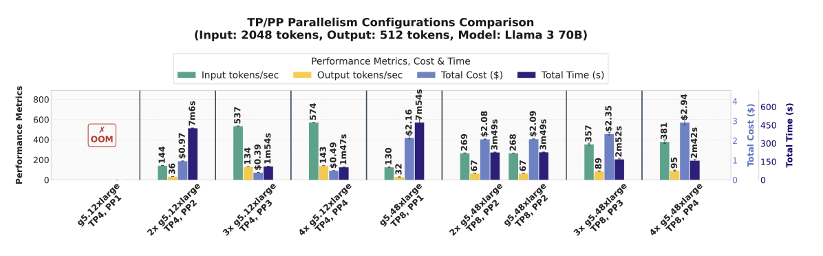 Figure 1. Input/output throughput (green/yellow bars, left axis), total dollar cost for the 30-request benchmark (light blue, inner-right axis), and total wall-clock runtime (dark blue, far-right axis). Total eight feasible configurations: TP={4,8} × PP={1,2,3,4}.
Lesson one: More GPUs does not mean higher throughput
Concretely: TP=4, PP=4 uses 16 GPUs and delivers 717 tok/s. TP=8, PP=4 uses 32 GPUs — twice as many — and delivers only 476 tok/s. Doubling the GPU count cut throughput by a third.
The same pattern holds across the whole TP=8 branch: at matched PP, TP=8 delivers lower absolute throughput than TP=4 despite running on 2× the hardware. You can literally buy more GPUs and get less inference done.
In other words, the $/token optimal point is not the same as the throughput optimal point.
The throughput winner is TP=4, PP=4 at 717 tok/s — but it costs $6.35 per million tokens. The $/token winner is TP=4, PP=3 at 671 tok/s and $5.09 per million tokens: 7% slower, 20% cheaper per token. Pick the throughput winner by default and you pay roughly 25% more per token for a speed gain nobody asked for.
Lesson two: Sublinear, linear, and superlinear scaling all exist
From TP=4, PP=2 to TP=4, PP=3, the throughput scales superlinearly. 180 → 671 tok/s while GPU count goes 8 → 12 — that is 3.7× more throughput for 1.5× more hardware, or 248% of ideal linear scaling. The mechanism: at PP=2 the pipeline is too shallow to amortize its bubble cost; at PP=3 it finally fills and the overlap benefit kicks in.
From TP=4, PP=3 to TP=4, PP=4, the throughput scales sublinearly. 671 → 717 tok/s for 12 → 16 GPUs — 7% more throughput for 33% more GPUs.
From PP=3 to PP=4, throughput stays almost the same. It is pure waste of money. This holds in both branches: TP=4 goes 671 → 717 (+7%), TP=8 goes 446 → 476 (+7%) — each time for 33% more GPUs. You pay for the fourth node and you get almost nothing.
From {TP=4,PP=3} to {TP=8,PP=3}, surprisingly, the absolute throughput sometimes goes down. TP=4 PP=3 on 12 GPUs delivers 671 tok/s; TP=8 PP=3 on 24 GPUs delivers 446 tok/s — twice the hardware, 33% less output. This is exactly the pathology Lesson one warned about.
Lesson three: The optimal configuration changes with requirements
Maximizing throughput? Minimizing absolute cost? Minimizing $/token? Meeting a specific SLO? Different requirements lead to different optimal configurations.
For this fixed workload (30 requests, 2,048-in / 512-out):
| Objective | Winning configuration | Result |
|---|---|---|
| Max throughput | TP=4, PP=4 on 4× g5.12xlarge | 717 tok/s, runtime 1m47s, $0.49 total, $6.35 per million tokens |
| Min absolute cost | TP=4, PP=3 on 3× g5.12xlarge | $0.39 total for the 30-request benchmark |
| Min $/token | TP=4, PP=3 on 3× g5.12xlarge | $5.09 per million tokens |
The min-absolute-cost and min-$/token configs are the same here because the workload size is fixed. That equivalence breaks as soon as the workload shape or request count changes, since cost has a fixed provisioning component and a variable serving component that scale differently.
Three different objectives, two different winning configs. Change the objective and the "right" config flips — and we have not even varied the workload shape yet. The premise that you can pick a config once and forget it already breaks down on this one workload.
Scaling efficiency and cost efficiency
As long as it satisfies the SLO, the optimal configuration will be the one that minimizes $/token. Let's see how the throughput scaling efficiency and cost efficiency look.
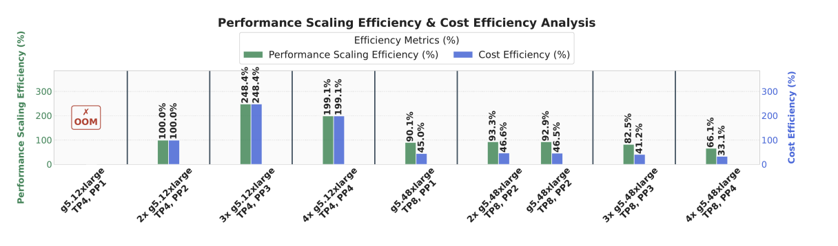 Figure 2. Performance scaling efficiency (green, left) and cost efficiency (blue, right), both normalized to 2× g5.12xlarge TP=4 PP=2 = 100%. Scaling efficiency is throughput gain per GPU added relative to the reference; cost efficiency is throughput-per-dollar-per-hour relative to the reference.
The efficiency view normalizes everything to 2× g5.12xlarge TP=4 PP=2 as 100%.
For TP=4, which has the best Pareto frontier, efficiency peaks at PP=3 and then goes down at PP=4.
TP=4 PP=3 scores 248% scaling efficiency — going from 2 nodes to 3 did not deliver the expected 1.5× throughput, it delivered roughly 2.5×. That is superlinear, and it is not a measurement artifact. It happens because at PP=2 the prefill phase is not long enough to keep both pipeline stages busy — you pay the full pipeline-bubble cost and get none of the overlap benefit. At PP=3, the pipeline depth finally matches the workload and the overlap starts working. At PP=4, you have overshot, and scaling drops back to sublinear (199%).
The TP=8 branch tells a different story. Scaling efficiency sits between 66% and 93% — not catastrophic. But cost efficiency collapses to 33–47%. Because g5.48xlarge costs roughly 4× more per hour than g5.12xlarge, even a TP=8 config running at 93% scaling efficiency delivers tokens at less than half the reference's cost efficiency.
For this workload on A10G, TP=8 is structurally doomed: you pay more per hour for hardware that does comparable or worse work. To understand why TP=8 is so bad for this deployment scenario, it needs one layer deeper analysis. We will dive deep to see why in a future post.
Remember: when you are buying more GPUs and getting the same throughput, you are throwing away money for nothing. The scary part is that there is a high chance you do not know whether you are throwing away your money or not.
GPU utilization
This is where the common intuition about GPU utilization breaks.
GPU utilization has often been considered the north-star metric to measure how efficiently a cluster has been operated. No and no. Please forget about it. It is a metric that misleads you.
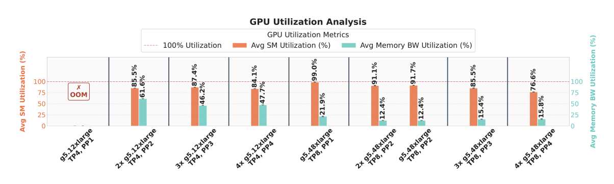 Figure 3. Average per-GPU streaming-multiprocessor utilization (orange, left) and average memory-bandwidth utilization (teal, right) across the sweep. The dashed line marks 100%. SM% near saturation means the compute units are running continuously; memory-BW% shows how much of peak HBM bandwidth is actually being used.
Higher GPU compute utilization does not mean higher throughput.
The highest SM utilization in the whole sweep is TP=8 PP=1 at 99%. Every A10G is computing continuously, at saturation. It is also the slowest configuration in the sweep at 7m54s, and one of the most expensive per token. If SM utilization measured useful work, this config would be the obvious winner. It is not.
The reason is right next to it on the plot: TP=8 PP=1's memory-bandwidth utilization is 21.9%. Decode is memory-bandwidth-bound — every generated token streams the model shard through HBM — so a configuration that is compute-saturated while the memory buses sit about 78% idle is a configuration spending its compute on the wrong thing. The SMs are running NCCL all-reduce kernels for every layer, not forward passes. Busy, but not productive.
Then, GPU memory bandwidth utilization?
No, higher GPU memory-bandwidth utilization also does not mean higher throughput or lower $/token. We saw that the highest throughput scalability and cost-efficiency configuration was TP=4 PP=3. It has 46% memory-bandwidth utilization, which is lower than TP=4 PP=2.
Maximizing cluster utilization is the wrong optimization. An intelligent system should optimize the performance objective — cost, throughput, $/token — directly, not indirectly through high utilization. Was the busy cycle in hardware doing useful work or not? You never know.
Takeaway from the A10G case study
One GPU type, one workload, eight configurations. The throughput range is 4.4× (162 → 717 tok/s). The cost range is 7.5× ($0.39 → $2.94). Scaling efficiency ranges 3.8× (66% → 248%). And the single highest-SM-utilization configuration is one of the worst on cost.
If you tried to pick the winner by reading the A10G datasheet and doing roofline math, you would not land on 3× g5.12xlarge TP=4 PP=3 — but that is, unambiguously, the right answer for this workload.
And this is one slice — one GPU, one workload, one model. The real problem expands along every other axis: different GPU types, different workload shapes, different models, different engine versions. Each one opens another matrix to search, and each one shifts the cost-optimal config.
This is what we are solving
This is the problem we are building Tandemn to solve. We treat it the way the data says it actually behaves: every production deployment is a measurement, and knowledge accumulates across deployments.
This is not the familiar "operators need better defaults" observation. It is that cost-optimal LLM inference is a live, ongoing optimization problem hiding inside every serving bill — and the industry is mostly paying the penalty for treating it as a one-shot configuration choice made under deadline pressure.
Copy status